111

DESIGN AND ANALYSIS OF BIOLOGICAL ASSAYS

Change to read:

INTRODUCTION

The potency of several Pharmacopeial articles must be determined by bioassays. The aim of this chapter is to present a concise account of certain essential biometrical procedures for bioassays in chapters or monographs of USP–NF, namely outlier identification, confidence intervals for relative potency measurements, and combination of independent assays. For bioassays not in USP–NF, other methods may be appropriate. See general information chapter Analysis of Biological Assays

1034

which may be a helpful, but not mandatory, guidance.

REJECTION OF OUTLYING OR ABERRANT OBSERVATIONS

A response that is questionable because of failure to comply with the procedure during the course of an assay is rejected. Other aberrant values may be discovered only after the responses have been tabulated, but can then be traced to assay irregularities that justify their omission. The arbitrary rejection or retention of an apparently aberrant response can be a serious source of bias. In general, the rejection of observations solely on the basis of their relative magnitudes, without investigation as to cause, is a procedure to be used sparingly. Should it be understood, either following an investigation into cause or based on practical assay experience, that an observation's discordance is unlikely to arise from a reasonable expectation of response to assay treatments, then a suspected aberrant response or outlier may be tested against one of two criteria, both of which assume that the data have an approximately normal distribution (which may be satisfied only after a suitable transformation of the original responses). Alternative statistically sound approaches to outlier detection may be used. The conditions under which outlier testing will be conducted and the criterion to be used should be specified a priori in the lab's procedures if not specified in the monograph or chapter.

Criterion 1 (Dixon's Test)

The first criterion is based on the variation within a single group of supposedly equivalent responses, such as a group of animals given a common concentration of a sample. At a confidence level of 99%, a valid observation will be rejected once in 100 trials (when the suspected outlier can occur at only one end) or once in 50 trials (when the suspected outlier can occur at either end), provided that relatively few, if any, responses within the group are identical. Arrange the responses in order of magnitude from y1 to yN, where N is the number of observations in the group. Compute the relative gap by using the formulas in Table 1 below.

Table 1

Sample Size (N)	Candidate Outlier is Smallest (y1)	Candidate Outlier is Largest (yN)
3–7	G1 = (y2 y1)/(yN y1)	G1 = (yN yN1)/(yN y1)
8–10	G2 = (y2 y1)/(yN1 y1)	G2 = (yN yN1)/(yN y2)
11–13	G3 = (y3 y1)/(yN1 y1)	G3 = (yN yN2)/(yN y2)

If G1, G2, or G3, as appropriate, exceeds the critical value in Table 2, for the observed N, there is a statistical basis for identifying the discordant measurement as an outlier and considering its removal. For N larger than 13, use Criterion 2.

In samples from a normal population, at a confidence level of 99%, gaps equal to or larger than the following values of G1, G2, and G3 occur with a probability P = 0.01, when outlier measurements can occur only at one end; or with P = 0.02, when they may occur at either end.

Table 2. Test for Outlier Measurements

N	3	4	5	6	7
G1	0.988	0.889	0.780	0.698	0.637

N	8	9	10	—	—
G2	0.683	0.635	0.597	—	—

N	11	12	13	—	—
G3	0.679	0.642	0.615	—	—

Criterion 2 (Grubbs, Extreme Studentized Deviate Test)

The second criterion may be used to examine for outlying values in groups of supposedly equivalent responses and may also be used in examining the set of residuals from a fitted model (linear or nonlinear) where there is constant variance. The final model (which yields the residuals for outlier detection) should include all important design variables. (For further discussion of design variables, see general information chapter Design and Development of Biological Assays

1032

, which may be a helpful, but not mandatory, resource.) (Note that for application to residuals, the following is an approximation. If the statistical software provides studentized residuals, those values should be used instead of those from the following equation.) For the value, R, that is furthest from the sample mean, compute the standardized deviation Z:

Z = (R

R)/S

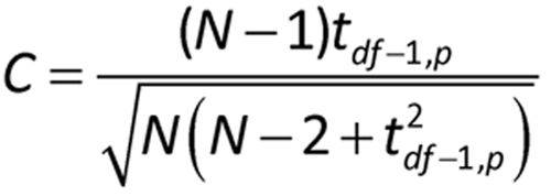
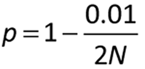
where R and S are the mean and standard deviation, respectively, of the set of values. For residuals from a least squares fit, such as for a parallel line assay, R = 0, and S is the square root of the residual mean square from the analysis. If |Z| is greater than C as determined below, then the value R is identified as a statistical outlier at the 1% level.

where N is the sample size, t is the one-sided 100p percentage point from the t distribution with df the degrees of freedom associated with S:

Alternative outlier methods are available that are intended for use on data sets that may contain multiple outliers and for detection of outliers associated with the bioassay design or model. For further discussion of outliers, see general information chapter Analytical Data—Interpretation and Treatment

1010

, which may be a helpful, but not mandatory, resource.

THE CONFIDENCE INTERVAL AND LIMITS OF POTENCY

The following method (Fieller's) is used to determine the confidence interval for an estimate of log relative potency from a parallel line assay or a slope ratio assay. Let M = a/b be the ratio for which we need a confidence interval. For the estimates, a and b, we have their respective standard errors, SEa and SEb, and a covariance between them, denoted Cov. The confidence interval, (MLow, MUp), for the estimated log relative potency then is as follows:

where:

and t = tdf,

/2 is the upper

/2 percentage point (or the two-sided

percentage point) with the residual degrees of freedom, df, from the statistical analysis and chosen confidence level, 100*(1

), (usually 95%). If g

1, it means that the denominator, b, is not statistically significantly different from 0 and the use of the ratio is not sensible for those data. The length, L, of this confidence interval is MUp

MLow.

For those cases in which the estimates of a and b are statistically uncorrelated (Cov = 0), the confidence interval formula simplifies to the following:

For further discussion of confidence intervals for potency, see chapter

1034

which may be a helpful, but not mandatory, resource.

COMBINATION OF INDEPENDENT ASSAYS

When the monograph or chapter permits, multiple independent assays may be performed until the combined results reduce the confidence interval width to within the limits specified in the pertinent monograph or chapter. Where two or more independent assays are required, each leading to a log-potency M, the M's are combined using one of the following two methods.

Method 1

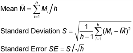
Let Mi denote the logarithm of the relative potency of the ith assay of h assay results to be combined. To combine the h results, the mean, standard deviation, and standard error of the Mi are calculated in the usual way:

A 100(1

)% confidence interval is then found as:

where th

/2 is the upper

/2 percentage point (or the two-sided

percentage point) of a t-distribution with h

1 degrees of freedom. The width, L, of this interval is 2th

/2SE.

Method 2

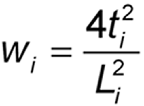
It is assumed that the results of each of the h assays have been analyzed to give h values of log potency with associated confidence limits. For each assay, i, obtain the confidence interval for the log potency or log relative potency. Then compute value Li by subtracting the ith lower confidence limit from the ith upper confidence limit. A weight wi for each value of the log relative potency, Mi, is calculated as follows, where ti has the same t-distribution value as that used in the calculation of confidence limits in the ith assay and is based on ni degrees of freedom:

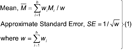
The products wiMi are formed for each assay, and their sum is divided by the total weight (w) for all assays to give the weighted mean log relative potency and its standard error as follows:

Next compute an approximate chi-square:

If the value of the approximate

2M is well under the 5% value shown in Table 3, compute the confidence interval using the mean and approximate standard error equations in (1) above; otherwise use Alternate weights as described below. Labs need to specify in their procedures how to quantify “well under”. Absent such a specification, the 20% values of Table 3 are suggested.

A 100(1

)% confidence interval in the log scale is then found as:

M ± L/2

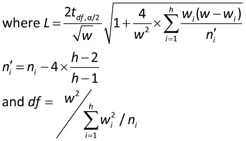
where tN,

/2 is the upper

/2 percentage point (or the two-sided

percentage point) of a t-distribution with degrees of freedom, df. The width of this interval is L.

Table 3. Critical Values for Approximate Chi-Square Test

	Critical Values
h	5%	20%
2	3.841	1.642
3	5.991	3.219
4	7.815	4.642
5	9.488	5.989
6	11.070	7.289
7	12.592	8.558
8	14.067	9.803
9	15.507	11.030
10	16.919	12.242

Alternate weights: The observed variation among the estimated log potencies or relative potencies can be divided into two components:

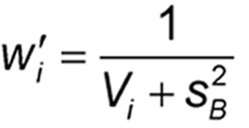
intra-assay variation for assay i:Vi = 1/wi
inter-assay component of variation:

For each assay, a weighting coefficient is then calculated as:

The confidence interval is then found as:

and t, the t-distribution value, is often approximated by the value 2.

For further discussion of combination of assays, see

1034

, which may be a helpful, but not mandatory, resource.

APPENDIX—KEY LITERATURE

Bliss, CI. Analysis of the biological assays in USP XV. Drug Standards, 24, 33–67, 1956.

Böhrer A. One-sided and two-sided critical values for Dixon's outlier test for sample sizes up to n = 30. Economic Quality Control 23, 5–13, 2008.

Cochran, WG. The combination of estimates from different experiments. Biometrics 10, 101–129, 1954.

Fieller, EC. Some problems in interval estimation. Journal of the Royal Statistical Society, B 16, 175–185, 1954.

Iglewicz, B and Hoaglin, DC. How to Detect and Handle Outliers. Quality Press, Milwaukee, 1993.

2S (USP38)

Auxiliary Information— Please check for your question in the FAQs before contacting USP.

Topic/Question	Contact	Expert Committee
General Chapter	Maura C Kibbey, Ph.D. Senior Scientific Liaison, Biologics & Biotechnology (301) 230-6309	(STAT2010) Statistics 2010

USP38–NF33 Page 176

USP38–NF33 Supplement : No. 2 Page 7576

Pharmacopeial Forum: Volume No. 40(4)